


Six tips for working with Excel 2010
With the introduction of the Ribbon in 2007, many familiar ways of interacting with Excel became hard to find while powerful new tools cropped up. These six tips can help you get the most out of the new interface and features and locate your old favorites.
Hide the Ribbon
Ribbon taking up too much screen space? You can temporarily turn it off. Doing this will get you back plenty of screen real estate, as you can see in the screenshot below.

It's easy to make the Ribbon disappear and reappear.
To hide the Ribbon, you can either press Ctrl-F1 (and press Ctrl-F1 again to make the Ribbon reappear) or just right-click anywhere in the Ribbon and select "Minimize the Ribbon."
The Ribbon will still be available when you want it -- all you need to do is click on the appropriate tab (Home, Insert, Page Layout, etc.) and it appears. It then discreetly goes away when you are no longer using it.
Add commands to the Quick Access toolbar
By letting you customize the Ribbon, Excel 2010 has gotten a lot more flexible than Excel 2007. But it can still be helpful to customize the Quick Access toolbar for one-click access to your most frequently used commands, no matter which Ribbon tab is showing.
As mentioned earlier in the story, you can do this via Backstage's Options screen, but a quicker way is to click the small down arrow to the right on the Quick Access toolbar and choose More Commands.
From the left-hand side of the screen that appears, choose commands that you want to add to the toolbar and click Add. You can change the order in which the buttons appear on the toolbar by highlighting a button on the right side of the screen and using the up and down arrows to move it.
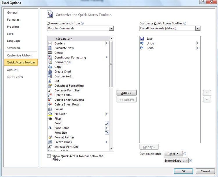
Adding buttons to the Quick Access toolbar. (Click image to enlarge.)
The list of commands you see on the left may seem somewhat limited at first. That's because Excel is showing you only the most popular commands. Click the drop-down menu under "Choose commands from" at the top of the screen, and you'll see other lists of commands -- All Commands, Home Tab and so on. Select any option, and there will be plenty of commands you can add.
Finally, there's an even easier way to add a command. Right-click any object on the Ribbon and choose "Add to Quick Access Toolbar." You can add not only individual commands in this way, but also entire groups -- for example, the Sparklines group.
Share Slicers across PivotTables
Here's a nifty Slicer trick: You can tie the same Slicer to multiple PivotTables so that, for example, you could select the West region in a Slicer and all connected PivotTables would filter their respective data on the same field. You can even make this work when the PivotTables are on different workbooks. Here's how to do it:
1. Create your first PivotTable on a workbook and define a Slicer: Click anywhere inside the PivotTable. Excel adds a PivotTable Tools tab to the Ribbon. Choose the Options subtab, and in the Ribbon that appears, click on the Insert Slicer icon (do not click the down-pointing arrow that reads "Insert Slicer" -- we'll cover that option in a moment).
2. Choose the field you want to filter from the list of fields in your PivotTable, then choose OK. Repeat for each Slicer you want to create.
3. Create another PivotTable on the same worksheet. This PivotTable must have a field with the same name as the field in the first PivotTable for which you created the Slicer in Step 2. Click anywhere within this second PivotTable, then once again choose the Options subtab from the PivotTable Tools tab. This time, however, choose the down-pointing arrow that reads "Insert Slicer" and choose "Slicer Connections..."
4. Excel displays a list of Slicers from the first PivotTable. Check the boxes for the Slicers you want to apply to your second PivotTable and choose OK. Check to see that the Slicer filters data in both PivotTables simultaneously.

The dialog box lets you apply a Slicer from one PivotTable to a second PivotTable. Once this is enabled, choosing a month will update both tables at the same time. (Click image to enlarge.)
5. Copy and paste your second PivotTable to a new worksheet. The connection to the original Slicer is still intact. You can now delete the second PivotTable from the original worksheet.
Note: Before moving on to Step 5, be sure to connect all the Slicers you want to work with your second PivotTable in Step 4. If you decide that you want to add another Slicer after you've already moved the second PivotTable to another worksheet, you'll have to go back to Step 3 and start again on the original worksheet.
Find your old friends
If you've been using Excel 2007, you've probably found most of the features and functions you used in earlier versions of Excel. But if you're upgrading directly to Excel 2010 from Excel 2003 or earlier, you may have a harder time locating many of your favorite commands.
Use our for an extensive list of where to find your old friends in the newest version of Excel. To save you more time, we've also included keyboard shortcuts for all these commands.
Use macros
As in Excel 2007, macros -- ingenious shortcuts you can create for performing repetitive tasks -- are hard to find in Excel 2010. But they're there: If you display the Developer tab, you'll find the macro tools in all their glory in the Code group. In fact, they're easier to reach than they were in earlier versions of Excel.

All your macro controls are in the Code group on the Developer tab.
You'll find everything you want in the Code group. Record a macro by clicking the Record Macro button, manage your macros by clicking the Macros button, and configure security for a macro by clicking the Macro Security button.
(Bonus bug fix: Unlike in Excel 2007, recording a macro when formatting a chart in Excel 2010 will now actually produce macro code.)
Use keyboard shortcuts
If you've been using keyboard shortcuts in Excel 2007, Excel 2003 or earlier versions, take heart -- most of the same ones work in Excel 2010. Any shortcuts that use the Ctrl key, such as Ctrl-C for copying to the clipboard and Ctrl-V for pasting, still work. And most of the old Alt-key shortcuts work as well, although not every one of them. See the table at the bottom of the page for the most useful shortcuts in Excel.
You can also use a clever set of keyboard shortcuts for working with the Ribbon. (These are unchanged from Excel 2007.) Press the Alt key, and then a tiny letter or number icon will appear on the menu for each tab -- for example, the letter H for the Home tab. Now press that letter on your keyboard, and you'll display that tab or menu item. When the tab appears, there will be letters and numbers for most options on the tab as well.
Once you've started to learn these shortcuts, you'll naturally begin using key combinations. So instead of pressing Alt then H to display the home tab, you can press Alt-H together.
The screenshot above shows the most useful Alt key combinations in Excel 2010. For more nifty keyboard shortcuts, see the table below. And even more shortcuts are listed on Microsoft's Office 2010 site.
Next:
More useful keyboard shortcuts in Excel 2010
| Key combination | Action |
|---|---|
| Worksheet navigation | |
| PgUp / PgDn | Move one screen up / down |
| Alt-PgUp / Alt-PgDn | Move one screen to the left / right |
| Ctrl-PgUp / Ctrl-PgDn | Move one worksheet tab to the left / right |
| Tab | Move to the next cell to the right |
| Shift-Tab | Move to the cell to the left |
| Home | Move to the beginning of a row |
| Ctrl-Home | Move to the beginning of a worksheet |
| Ctrl-End | Move to the last cell that has content in it |
| Ctrl-Left arrow | Move to the word to the left while in a cell |
| Ctrl-Right arrow | Move to the word to the right while in a cell |
| Ctrl-G or F5 | Display the Go To dialog box |
| F6 | Switch between the worksheet, the Ribbon, the task pane and Zoom controls |
| Ctrl-F6 | If more than one worksheet is open, switch to the next one |
| Working with data | |
| Shift-Spacebar | Select a row |
| Ctrl-Spacebar | Select a column |
| Ctrl-A or Ctrl-Shift-Spacebar | Select an entire worksheet |
| Shift-Arrow key | Extend selection by a single cell |
| Shift-PgDn / Shift-PgUp | Extend selection down one screen / up one screen |
| Shift-Home | Extend selection to the beginning of a row |
| Ctrl-Shift-Home | Extend selection to the beginning of the worksheet |
| Ctrl-C | Copy cell's contents to the clipboard |
| Ctrl-X | Copy and delete cell's contents |
| Ctrl-V | Paste from the clipboard into a cell |
| Ctrl-Alt-V | Display the Paste Special dialog box |
| Enter | Finish entering data in a cell and move to the next cell down |
| Shift-Enter | Finish entering data in a cell and move to the next cell up |
| Esc | Cancel your entry in a cell |
| Ctrl-; | Insert the current date |
| Ctrl-Shift-; | Insert the current time |
| Ctrl-K | Insert a hyperlink |
| Ctrl-T or Ctrl-L | Display the Create Table dialog box |
| Formatting cells and data | |
| Ctrl-1 | Display the Format Cells dialog box |
| Alt-' | Display the Style dialog box |
| Ctrl-Shift-& | Apply a border to a cell or selection |
| Ctrl-Shift-_ | Remove a border from a cell or selection |
| Ctrl-Shift-$ | Apply the Currency format with two decimal places |
| Ctrl-Shift-~ | Apply the Number format |
| Ctrl-Shift-% | Apply the Percentage format with no decimal places |
| Ctrl-Shift-# | Apply the Date format using day, month and year |
| Ctrl-Shift-@ | Apply the Time format using the 12-hour clock |
| Working with formulas | |
| = | Begin a formula |
| Alt-= | Insert AutoSum |
| Shift-F3 | Display the Insert Function dialog box |
| Ctrl-` | Toggle between displaying formulas and cell values |
| Ctrl-' | Copy and paste the formula from the cell above into the current one |
| F9 | Calculate all worksheets in all workbooks that are open |
| Shift-F9 | Calculate the current worksheet |
| Other useful shortcuts | |
| Ctrl-N | Create a new workbook |
| Ctrl-O | Open a workbook |
| Ctrl-S | Save a workbook |
| Ctrl-W | Close a workbook |
| Ctrl-P | Print a workbook |
| Ctrl-F | Display the Find and Replace dialog box |
| Shift-F2 | Insert or edit a cell comment |
| Ctrl-Shift-O | Select all cells that contain comments |
| Ctrl-9 | Hide selected rows |
| Ctrl-Shift-9 | Unhide hidden rows in a selection |
| Ctrl-0 | Hide selected columns |
| Ctrl-Shift-0 | Unhide hidden columns in a selection |
| Ctrl-Z | Undo the last action |
| Ctrl-Y | Redo the last action |
Preston Gralla is a contributing editor for Computerworld and the author of more than 35 books, including How the Internet Works (Que, 2006).
Rich Ericson is a Northwest-based technology writer and the reviews editor of The Office Letter, a site devoted to tips for Microsoft Office.